🌬️🍃 Week 8 Lab: Matching & Instrumental Variable Estimation

Author

EDS 241

Published

February 25, 2025

A replication of IV analyses from study:

Stokes (2015): “Electoral Backlash against Climate Policy: A Natural Experiment on Retrospective Voting and Local Resistance to Public Policy.

Study: https://doi.org/10.1111/ajps.12220
Data source: Dataverse-Stokes2015

NOTE: Replication of IV results is approximate. An alternative matching procedure was followed in this class exercise for illustration purposes.

Setup - Load libraries & data

library(tidyverse)
library(janitor)
library(here)         
library(gt)
library(gtsummary)
library(jtools) 
library(AER)        # 2SLS
library(MatchIt)    # Matching
library(cobalt)     # Balance & love plots
library(DiagrammeR) # Path diagrams

clean_data <- read_csv(here("data", "stokes15_ivdata.csv")) %>%
  mutate(across(c(precinct_id, district_id), as.factor))

Intuition check - Why match?

clean_data %>%
    select(proposed_turbine_3km, log_home_val_07, p_uni_degree, log_median_inc, log_pop_denc) %>%
    tbl_summary(
        by = proposed_turbine_3km,
        statistic = list(all_continuous() ~ "{mean} ({sd})")) %>%
    modify_header(label ~ "**Variable**") %>%
    modify_spanning_header(c("stat_1", "stat_2") ~ "**Treatment**")

Variable	Treatment
Variable	0 N = 5,619¹	1 N = 354¹
log_home_val_07	12.26 (0.37)	12.29 (0.29)
p_uni_degree	0.17 (0.12)	0.13 (0.09)
log_median_inc	10.32 (0.22)	10.31 (0.19)
log_pop_denc	5.12 (2.40)	3.54 (1.78)
¹ Mean (SD)

What type of data do I need for matching?

Multiple covariates/controls (wide data)
Extra control observations (large comparison group)

Tip

Be cautious when choosing controls to avoid accidentally controlling away the treatment effect!

The rationale for matching as described in Stokes, 2015:

“Using matching to preprocess the data before using an instrumental variable estimator may strengthen the instrument and correct for biases from confounders if the instrument departs from as-if random assignment (Keele and Morgan 2013).
[…]
Mahalanobis distance matching was first used to pair each treated unit with a control unit based on observable characteristics. The data were balanced on four variables: the average home price pretreatment in 2006 (log), the population with a university degree (%), median income (log), and population density (log).”

Conduct matching estimation using the {`MatchIt`} 📦

📜 Documentation - MatchIt

Approximate Mahalanobis matching method used in Stokes (2015)
Introduce another very common matching approach called propensity score matching

NOTE: In the replication code associated with Stokes (2015) the {AER} package is used for Mahalanobis matching. In this tutorial we utilize the {MatchIt} package for this class exercise. The results are comparable but not exactly the same.

set.seed(02252025)

match_model <- matchit(
     proposed_turbine_3km ~ # TREATMENT
     log_home_val_07 + p_uni_degree + log_median_inc + log_pop_denc, # Pre-treatment covariates
  data = clean_data, 
  method = "nearest",       # Nearest neighbor matching
  distance = "mahalanobis", # Mahalanobis distance
  ratio = 1,                # Match one control unit to each treatment (1-to-1 matching)
  replace = FALSE           # Control obs. are not replaced
)

# Extract matched data
matched_data <- match.data(match_model)

summary(match_model)

❤️ ️Create a “love plot” using `love.plot()`

📜 Documentation - cobalt

Plot mean differences for data before & after matching across all pre-treatment covariates
This is an effectives way to evaluate pre-treatment balance!

new_names <- data.frame(
    old = c("log_home_val_07", "p_uni_degree", "log_median_inc", "log_pop_denc"),
    new = c("Home Value (log)", "Percent University Degree", "Median Income (log)", "Population Density (log)"))

# Love plot
love.plot(match_model, stats = "mean.diffs", 
          thresholds = c(m = 0.1), 
          var.names = new_names)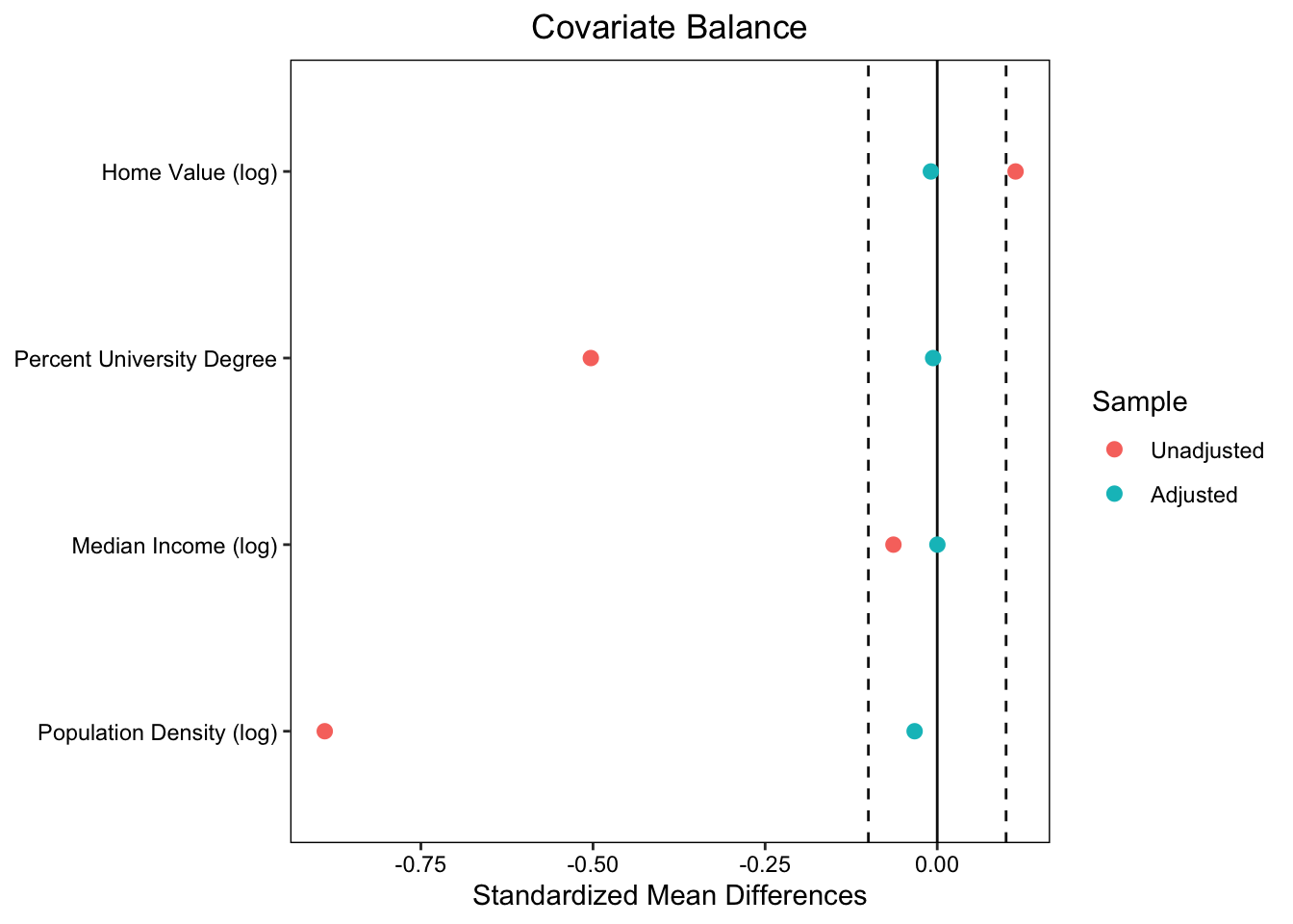

Propensity score matching

propensity_scores <- matchit(
  proposed_turbine_3km ~ 
      log_home_val_07 + p_uni_degree + log_median_inc + log_pop_denc,
  data = clean_data, 
  method = "nearest", # Nearest neighbor matching
  distance = "logit", # Propensity scores estimated with logistic regression
  ratio = 1,          # Match one control unit to each treatment (1-to-1 matching)
  replace = FALSE     # Control obs. are not replaced
)

Create table displaying covariate balance using `cobalt::bal.tab()`

bal.tab(propensity_scores, 
        var.names = new_names)

Balance Measures
                    Type Diff.Adj
distance        Distance   0.0001
log_home_val_07  Contin.   0.0205
p_uni_degree     Contin.   0.0457
log_median_inc   Contin.  -0.0042
log_pop_denc     Contin.  -0.0365

Sample sizes
          Control Treated
All          5619     354
Matched       354     354
Unmatched    5265       0

Simulate matching in 241 - Find your counterfactual!

Covariates:

Hair color: Black, Brown, Blonde, Red
Eye color: Brown, Blue, Green, Hazel
Handedness: Right-handed, Left-handed

An ‘exact’ match = Someone who is matching on all 3 covariates. Find your closest match!

Instrumental Variable Estimation: Two-Stage Least Squares (2SLS)

First stage: Regress the treatment (\(X\)) on the instrument (\(Z\))

\[X_i = \alpha_0 + \alpha_1 Z_i + \mu_i\]

Fitted regression notation: (\(\hat{X}_i\)) indicates predicted values (i.e., `hat` \(\widehat{symbol}\))

\[\hat{X}_i = \hat{\alpha_0} + \hat{\alpha_1} Z_i\]

Second stage: Regress the outcome (\(Y\)) on the fitted values from the 1st stage (\(\hat{X}_i\))

\[Y_i = \beta_0 + \beta_1 \hat{X}_i + \epsilon_i\]

Replicating IV estimator in Stokes (2015) - “Table 2”

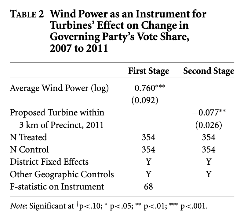
The 2SLS step-wise procedure

Step 1. Estimate the first stage regression equation

\[ProposedTurbine_i = \beta_0 + \beta_1 WindPower_i + ControlVariables... + \epsilon_i\] #### Control variables included in 1st & 2nd stage regressions:

Distance to lakes
District fixed effects
Flexible geographic controls

“Geographic controls, in both the first and second stage, included longitude, latitude, both variables squared, and their interaction.” (Stokes, 2015).

first_stage <- lm(proposed_turbine_3km ~  # TREATMENT
                      log_wind_power +    # INSTRUMENT
                      mindistlake + mindistlake_sq + # CONTROLS
                      longitude + latitude + long_sq + lat_sq + long_lat + # GEOGRAPHIC CONTROLS
                      district_id, # FIXED EFFECT
                  data=matched_data)

export_summs(first_stage, digits = 3,  model.names = c("First stage: Prpoposed Turbine 3km"),
             coefs = c("(Intercept)", "log_wind_power") )

	First stage: Prpoposed Turbine 3km
(Intercept)	15.027
	(74.243)
log_wind_power	0.711 ***
	(0.092)
N	708
R2	0.419
* p < 0.001; p < 0.01; * p < 0.05.

Check 1st stage for `relevance` - to make sure your instrument is not weak 🤕

General rule of thumb: F-statistic > 10 is considered a relevant instrument (Stock, Wright, & Yogo, 2020)

# `summary(first_stage)` # Includes the F-statistic at the bottom of long output table

summary(first_stage)$fstatistic

    value     numdf     dendf 
 14.70538  33.00000 674.00000

Step 2. Save predicted values \(\hat{X}_i\) from first stage

matched_data$proposed_turbine_3km_HAT <- predict(first_stage, newdata = matched_data)

Step 3. Estimate the second stage regression

\[LiberalVoteShare_i = \beta_0 + \beta_1 \widehat{ProposedTurbine}_i + ControlVariables... + \epsilon_i\]

second_stage <- lm(change_liberal ~ # OUTCOME
                       proposed_turbine_3km_HAT + # PREDICTED VALUES OF X (LATE)
                       mindistlake + mindistlake_sq +
                       longitude + long_sq + latitude + lat_sq + long_lat +
                       district_id, 
                   data = matched_data)

export_summs(second_stage, digits = 3,  model.names = c("Second stage: Change in Liberal Vote Share"),
             coefs = c("(Intercept)", "proposed_turbine_3km_HAT") )

	Second stage: Change in Liberal Vote Share
(Intercept)	16.966
	(15.432)
proposed_turbine_3km_HAT	-0.065 *
	(0.027)
N	708
R2	0.586
* p < 0.001; p < 0.01; * p < 0.05.

Local Average Treatment Effect (LATE)

The treatment effect for the `complier group` 🎟️ → 🍕

Recall that the 2SLS estimator estimates the LATE
Given that all of the identifying assumptions hold:
1. Instrument relevance ( the instrument is strong 💪 )
2. Exclusion assumption ( No Z on Y except through X ⛔️ )
3. Ignorability ( Z is ‘as if random’ with respect to Y 🎲 )
4. Monotonicity ( No defiers 🙃 )
Asssuming 1-4 2SLS will consistently return the LATE (i.e., the treatment effect among compliers)
Compliers = Participants who were encouraged by the instrument (🎟) to take the treatment (🍕)

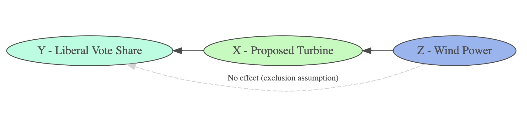
Illustrate the `exclusion assumption` using {`DiagrammeR`}

📜 Documentation - DiagrammeR

grViz("
  digraph path_diagram {
    # Graph layout settings
    rankdir = LR;  # Left-to-right layout

    # Node definitions
    node [shape = ellipse, style = filled, fillcolor = AquaMarine]
    Y_LiberalVoteShare [label = 'Y - Liberal Vote Share']
    
    node [shape = ellipse, style = filled, fillcolor = PaleGreen]
    X_ProposedTurbine [label = 'X - Proposed Turbine']
    
    node [shape = ellipse, style = filled, fillcolor = CornFlowerBlue]
    Z_WindPower [label = 'Z - Wind Power']

    # Reversed Edges (Directed Arrows)
    X_ProposedTurbine -> Z_WindPower [dir = back] 
    Y_LiberalVoteShare -> X_ProposedTurbine  [dir = back]
    Y_LiberalVoteShare -> Z_WindPower [label = 'No effect (exclusion assumption)',
    fontsize=10, style = dashed, color = gray, constraint = false, dir = back]
  }
")

Estimate 2SLS using `ivreg()` from {`AER`}

📜 Documentation - AER

Syntax for specify 2SLS using ivreg():

ivreg( Y ~ X | Z , data )

fit_2sls <- ivreg(change_liberal ~ # OUTCOME
                    proposed_turbine_3km + # TREATMENT 
                    mindistlake + mindistlake_sq + # CONTROLS
                    longitude + long_sq + latitude + lat_sq + long_lat + # CONTROLS
                    district_id |   # FIXED EFFECT 
                    log_wind_power + # INSTRUMENT
                    mindistlake + mindistlake_sq + # CONTROLS REPEATED...
                    longitude + long_sq + latitude + lat_sq + long_lat + 
                    district_id, 
                data = matched_data)

summary(fit_2sls)


Call:
ivreg(formula = change_liberal ~ proposed_turbine_3km + mindistlake + 
    mindistlake_sq + longitude + long_sq + latitude + lat_sq + 
    long_lat + district_id | log_wind_power + mindistlake + mindistlake_sq + 
    longitude + long_sq + latitude + lat_sq + long_lat + district_id, 
    data = matched_data)

Residuals:
       Min         1Q     Median         3Q        Max 
-0.3603355 -0.0479715  0.0006369  0.0509007  0.2750431 

Coefficients:
                       Estimate Std. Error t value Pr(>|t|)    
(Intercept)           1.697e+01  1.574e+01   1.078 0.281383    
proposed_turbine_3km -6.539e-02  2.742e-02  -2.384 0.017381 *  
mindistlake           1.564e-03  5.087e-04   3.074 0.002199 ** 
mindistlake_sq       -1.784e-05  4.441e-06  -4.016 6.58e-05 ***
longitude            -1.499e-01  3.136e-01  -0.478 0.632787    
long_sq              -2.469e-03  2.006e-03  -1.230 0.218973    
latitude             -1.077e+00  5.739e-01  -1.876 0.061025 .  
lat_sq                7.048e-03  6.578e-03   1.071 0.284350    
long_lat             -5.789e-03  3.825e-03  -1.513 0.130663    
district_id10         2.995e-01  5.112e-02   5.859 7.30e-09 ***
district_id14         4.630e-02  7.458e-02   0.621 0.534886    
district_id18         1.758e-01  6.372e-02   2.759 0.005947 ** 
district_id19         2.145e-01  6.371e-02   3.367 0.000804 ***
district_id21        -5.027e-02  7.222e-02  -0.696 0.486615    
district_id22         3.518e-03  7.835e-02   0.045 0.964198    
district_id28         1.616e-01  7.065e-02   2.287 0.022498 *  
district_id29         2.386e-01  6.114e-02   3.903 0.000105 ***
district_id34         1.451e-01  5.772e-02   2.514 0.012161 *  
district_id36         2.229e-01  9.010e-02   2.474 0.013588 *  
district_id40         7.669e-02  6.777e-02   1.132 0.258218    
district_id41         1.718e-01  8.254e-02   2.081 0.037797 *  
district_id42         1.776e-01  9.401e-02   1.889 0.059257 .  
district_id55         1.980e-01  7.017e-02   2.822 0.004914 ** 
district_id58         1.511e-01  7.002e-02   2.157 0.031337 *  
district_id67         1.350e-01  7.040e-02   1.918 0.055533 .  
district_id69         8.231e-02  4.923e-02   1.672 0.094973 .  
district_id70         1.381e-01  6.473e-02   2.133 0.033286 *  
district_id73         1.392e-01  7.247e-02   1.920 0.055257 .  
district_id85         1.518e-01  5.186e-02   2.928 0.003523 ** 
district_id87         1.317e-01  1.095e-01   1.203 0.229343    
district_id90        -3.282e-02  1.396e-01  -0.235 0.814148    
district_id91        -1.173e-01  1.280e-01  -0.916 0.359736    
district_id98         2.094e-01  7.557e-02   2.771 0.005748 ** 
district_id105        1.131e-01  6.646e-02   1.702 0.089206 .  
---
Signif. codes:  0 '***' 0.001 '**' 0.01 '*' 0.05 '.' 0.1 ' ' 1

Residual standard error: 0.08245 on 674 degrees of freedom
Multiple R-Squared: 0.5696, Adjusted R-squared: 0.5485 
Wald test: 27.81 on 33 and 674 DF,  p-value: < 2.2e-16

[1] "HUZZAH! 🚀 Great work 241 - You are phenomenal! 💫"


 --------- 
< The End >
 --------- 
      \
       \

         __
        /o \
      <=   |         ==
        |__|        /===
        |   \______/  =
        \     ====   /
         \__________/     [ab]

A replication of IV analyses from study:

Stokes (2015): “Electoral Backlash against Climate Policy: A Natural Experiment on Retrospective Voting and Local Resistance to Public Policy.

Setup - Load libraries & data

Intuition check - Why match?

What type of data do I need for matching?

Conduct matching estimation using the {MatchIt} 📦

❤️ ️Create a “love plot” using love.plot()

Propensity score matching

Create table displaying covariate balance using cobalt::bal.tab()

Simulate matching in 241 - Find your counterfactual!

Instrumental Variable Estimation: Two-Stage Least Squares (2SLS)

First stage: Regress the treatment (\(X\)) on the instrument (\(Z\))

Fitted regression notation: (\(\hat{X}_i\)) indicates predicted values (i.e., hat \(\widehat{symbol}\))

Second stage: Regress the outcome (\(Y\)) on the fitted values from the 1st stage (\(\hat{X}_i\))

Replicating IV estimator in Stokes (2015) - “Table 2”

The 2SLS step-wise procedure

Step 1. Estimate the first stage regression equation

Check 1st stage for relevance - to make sure your instrument is not weak 🤕

Step 2. Save predicted values \(\hat{X}_i\) from first stage

Step 3. Estimate the second stage regression

Local Average Treatment Effect (LATE)

The treatment effect for the complier group 🎟️ → 🍕

Illustrate the exclusion assumption using {DiagrammeR}

Estimate 2SLS using ivreg() from {AER}

Conduct matching estimation using the {`MatchIt`} 📦

❤️ ️Create a “love plot” using `love.plot()`

Create table displaying covariate balance using `cobalt::bal.tab()`

Fitted regression notation: (\(\hat{X}_i\)) indicates predicted values (i.e., `hat` \(\widehat{symbol}\))

Check 1st stage for `relevance` - to make sure your instrument is not weak 🤕

The treatment effect for the `complier group` 🎟️ → 🍕

Illustrate the `exclusion assumption` using {`DiagrammeR`}

Estimate 2SLS using `ivreg()` from {`AER`}