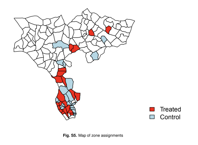
Map of Treatment Assignment Zones in Nansana, Uganda
Open source data & applied study:
Open access data was utilized for this class exercise from the study (Buntaine et al., 2024):
Buntaine, M. T., Komakech, P., & Shen, S. V. (2024). Social competition drives collective action to reduce informal waste burning in Uganda. Proceedings of the National Academy of Sciences, 121(23). https://doi.org/10.1073/pnas.2319712121
Goals of this exercise
Start with a simple OLS model
Demonstrate the rationale for estimating progressively complex models
Illustrate a causal inference approach (i.e., identify
robustestimators)Conclusion: What is the take-home message of the Lab-1 exercise? . . .
Estimating complex models is a relatively easy part of our work as data scientists…
- Making informed specification decisions & communicating results is the hard part (i.e., the science side of
data science)!
- Making informed specification decisions & communicating results is the hard part (i.e., the science side of
Let’s get started!
Load packages and data:
library(tidyverse)   # Keeping things tidy
library(janitor)     # Housekeeping
library(here)        # Location, location, location
#install.packages("jtools")
library(jtools)      # Pretty regression output
library(gt)          # Tables
library(gtsummary)   # Table for checking balance
#install.packages("performance")
library(performance) # Check model diagnostics
#install.packages("see") # Visualization engine for performance package
#install.packages("huxtable") # Package required for export_summs
# A tibble: 6 × 8
zoneid survey waste_piles rain_0_48hrs rain_49_168hrs pre_count_avg pair_id
<dbl> <chr> <dbl> <dbl> <dbl> <dbl> <dbl>
1 1011 post_tre… 97 0 0.4 97 2021
2 1012 post_tre… 12 0 0.4 12.5 2022
3 1013 post_tre… 58 0 0.4 87.5 2022
4 1014 post_tre… 88 0 0.4 110. 2021
5 1015 post_tre… 53 0.04 0.36 110. 2017
6 1016 post_tre… 18 0 0.4 23 2017
# ℹ 1 more variable: treat <dbl># Read in waste pile count data
counts_gpx <- read_csv(here::here( "data", "waste_pile_counts_gpx.csv")) %>%
rename("waste_piles" = "total",
"rain_0_48hrs" = "rf_0_to_48_hours",
"rain_49_168hrs" = "rf_49_to_168_hours") %>%
filter(survey%in%c(
"post_treatment_1","post_treatment_2","post_treatment_3",
"post_treatment_4","post_treatment_5"))
# Select subset of post-treatment periods
post_treat_subset <- counts_gpx %>%
filter(survey == "post_treatment_4")
head(post_treat_subset)Now that we got our data loaded in, lets take a look at what these variables mean.
| Label | Description |
|---|---|
| zoneid | Zone or neighborhood ID: The observational unit (\(N=44\)) |
| waste_piles | The outcome variable (\(Y\)): The number of waste pile burns recorded (Range: 5, 125) |
| treat | The treatment assignment variable (0 = Control Group; 1 = Treatment Group) |
| rf_0_to_48_hours | The rainfall estimated between 0 and 48 hours prior to the start of the audit, derived from NASA MEERA-2 corrected precipitation estimates (mm) |
| rf_49_to_168_hours | The rainfall estimated between 49 and 168 hours prior to the start of the audit, derived from NASA MEERA-2 corrected precipitation estimates (mm) |
| pre_count_avg | The average number of burnt piles in the pre-treatment audits, spread to zone level |
| pair_id | The unique ID assigned to each pair of zones for assignment to treatment |
Model 1: Simple OLS (Ordinary Least Squares) estimator
OLS estimator (specification):
\[waste\ piles =\beta_0 + \beta_1(treat) + \epsilon\]
m1_ols <- lm(
    waste_piles ~ treat,
    data = post_treat_subset)

summ(m1_ols, model.fit = FALSE)| Observations | 44 |
| Dependent variable | waste_piles |
| Type | OLS linear regression |
| Est. | S.E. | t val. | p | |
|---|---|---|---|---|
| (Intercept) | 77.91 | 4.16 | 18.73 | 0.00 |
| treat | -24.77 | 5.88 | -4.21 | 0.00 |
| Standard errors: OLS |
Are we making reasonable assumptions?
Remember questioning (and testing) assumptions is the heart of causal inference!We want to make sure our assumptions our reasonable. To do so, let’stake a quick look at our outcome variable waste piles, and then look at the normality of our residuals.
post_treat_subset %>%
  ggplot(aes(x = waste_piles)) +
  geom_histogram(binwidth = 5, fill = "blue", color = "white", alpha = 0.7) +
  labs(title = "Histogram of Waste Piles",
    x = "Waste Piles (counts)",
    y = "Count") +
    theme_minimal()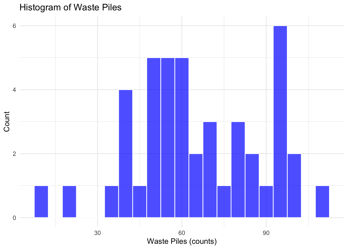
While our data isn’t a perfect bell curve, it also isn’t severely skewed. Let’s do another assumption check (normality of residuals) to help us decide if OLS is the right model for us.
To do so, we will make a QQ plot displaying residuals (y-axis) compared to the normal distribution (x-axis).
check_model(m1_ols, check = "qq" )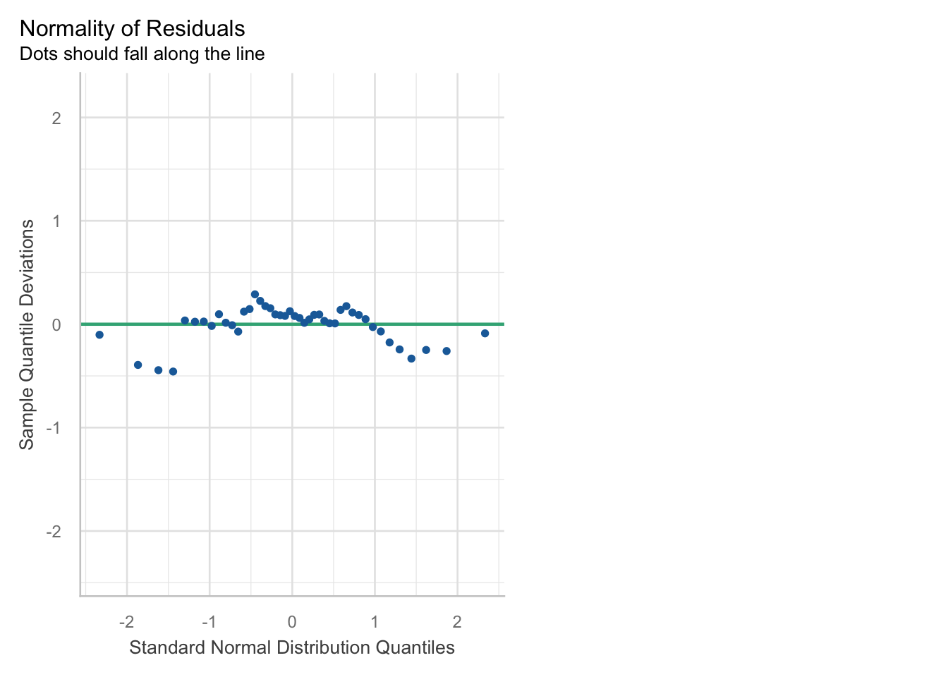
Hmm, it doesn’t seem like the OLS assumption, normality of residuals is a good fit for our data. Onto the next model!
TipDiscussion
Since we ruled OLS out, talk with your neighbor about another potential model to try. What kind of variable is our outcome variable? How might that inform what model we try next?
We can “relax” our assumptions by using a Generalized Linear model! Specifically, we will relax the assumption that the residuals are normally distributed.
WarningWarning!
When we relax an assumption and make our model more flexible, the statistics and interpretation become more complex!
As you discussed with your partner, our dependent variable, waste_piles is a count variable, not a continuous variable. Therefore, it’s best we pick a model that explicitly accounts for count outcomes. In walks the poisson regression model!
Model 2 : Poisson Generalized Linear Regression Model
We are going to assume Y follows a Poisson distribution with non negative integers (counts!). To do so, we need to think about the assumptions the Poisson regression makes. This model assumes that variance (dispersion) is proportional to the mean. Does our data match the theoretical distribution proposed? Let’s check!
lambda_hat <- mean(post_treat_subset$waste_piles)

poisson_curve <- tibble(
  x = seq(0, max(post_treat_subset$waste_piles), by = 1),  # Range of x values
  density = dpois(seq(0, max(post_treat_subset$waste_piles), by = 1),
                  lambda = mean(post_treat_subset$waste_piles))
)

ggplot(post_treat_subset, aes(x = waste_piles)) +
  geom_histogram(aes(y = ..density..), binwidth = 5, color = "white", fill = "blue", alpha = 0.7) +
  geom_line(data = poisson_curve, aes(x = x, y = density), color = "red", size = 1) +  # Poisson curve
  geom_density(color = "green", size = 1, adjust = 1.5) +  # KDE for a smoother curve
  labs(
    title = "Plot of Empirical (Green) v. Theoretical (Red) Distributions",
    x = "Waste Pile Counts",
    y = "Density"
  ) +
  theme_minimal()
m2_poisson <- glm(waste_piles ~ treat,
                  family = poisson(link = "log"),
                  data = post_treat_subset)

summ(m2_poisson, model.fit = FALSE)| Observations | 44 |
| Dependent variable | waste_piles |
| Type | Generalized linear model |
| Family | poisson |
| Link | log |
| Est. | S.E. | z val. | p | |
|---|---|---|---|---|
| (Intercept) | 4.36 | 0.02 | 180.32 | 0.00 |
| treat | -0.38 | 0.04 | -10.09 | 0.00 |
| Standard errors: MLE |
Just like OLS, we have some assumptions we need to check!
We first need to check for over dispersion. This is when our variance exceeds the mean.
check_overdispersion(m2_poisson)# Overdispersion test
dispersion ratio = 5.873
Pearson's Chi-Squared = 246.680
p-value = < 0.001If our dispersion ratio was equal to 1, this would mean our mean is equal to our variance. Since our dispersion ratio is 5.873, and far greater than 1, we can see that our data has significant overdispersion. Poisson isn’t the model for us!
TipDiscussion
Since we ruled OLS and Poisson Regression out, talk with your neighbor about another potential model to try.
Model 3: Log- OLS Regression
Log Linear Regression is an alternative way to model count outcomes using regular OLS. The only difference is that we are transforming our outcome variable to be on the log scale.
m3_log <- lm(
    log(waste_piles) ~ treat,
    data = post_treat_subset)

summ(m3_log, model.fit = FALSE)| Observations | 44 |
| Dependent variable | log(waste_piles) |
| Type | OLS linear regression |
| Est. | S.E. | t val. | p | |
|---|---|---|---|---|
| (Intercept) | 4.31 | 0.08 | 51.97 | 0.00 |
| treat | -0.42 | 0.12 | -3.57 | 0.00 |
| Standard errors: OLS |
We can compare our observed data to simulated data based on the model we just created (m3_log).
check_predictions(m3_log, verbose = FALSE)Warning: Minimum value of original data is not included in the
replicated data.
Model may not capture the variation of the data.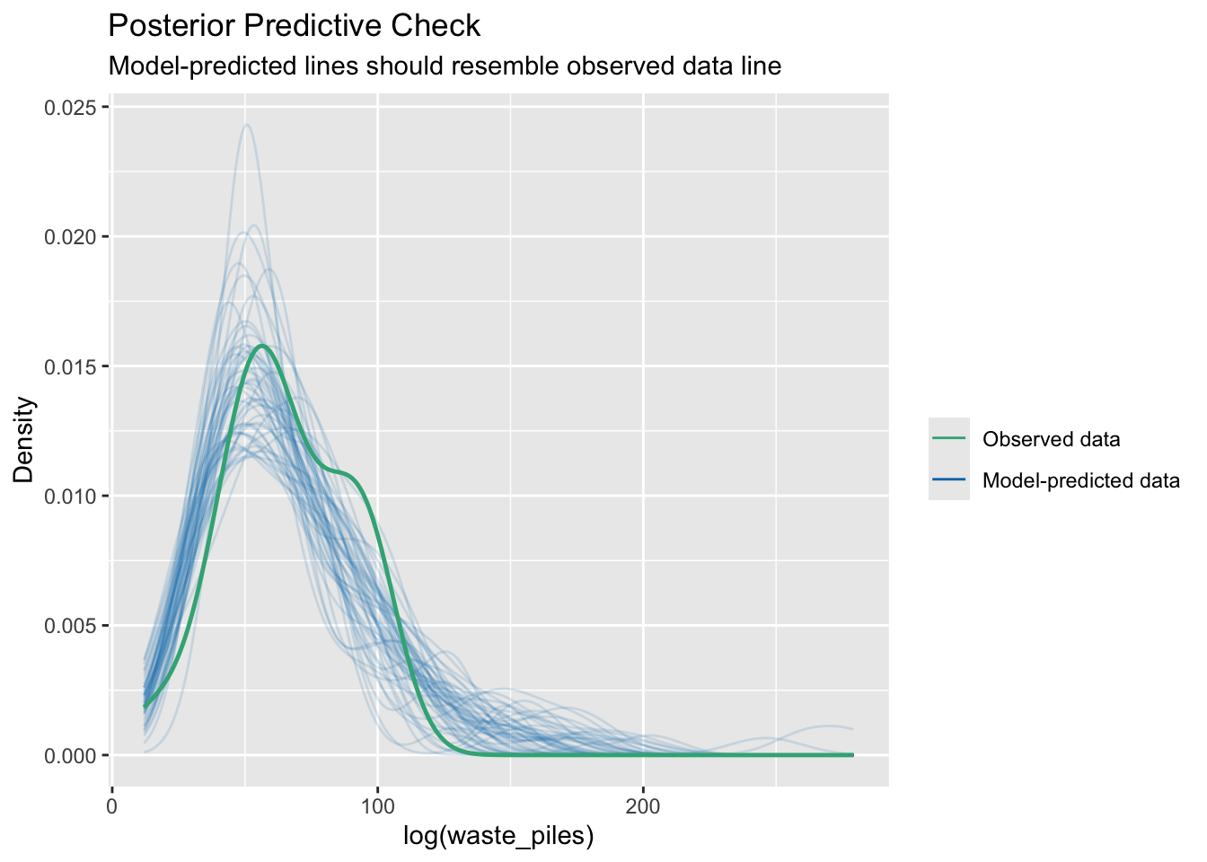
Model Recap
Let’s take a look at the three models we have created thus far and compare their results.
export_summs(m1_ols, m2_poisson, m3_log,
             model.names = c("OLS","Poisson GLM","Log(Outcome) OLS"),
statistics = "none")| OLS | Poisson GLM | Log(Outcome) OLS | |
|---|---|---|---|
| (Intercept) | 77.91 *** | 4.36 *** | 4.31 *** |
| (4.16) | (0.02) | (0.08) | |
| treat | -24.77 *** | -0.38 *** | -0.42 *** |
| (5.88) | (0.04) | (0.12) | |
| *** p < 0.001; ** p < 0.01; * p < 0.05. | |||
Let’s do some quick math to compare treatment effect estimates
\[\% \Delta Y = \left( e^{\beta_1} - 1 \right) \times 100\]
# Calculate percent change in waste piles in each model:

m1_change = (-24.77/77.91)*100   ## % change OLS = -31.8
m2_change = (exp(-.38) - 1)*100  ## % change POIS = -31.6
m3_change = (exp(-0.42) - 1)*100 ## % change LOG-OLS = -34.3
TipTreatment Estimate Check In
Interpret the treatment estimate for the log OLS.
The treatment estimate for log-OLS can be interpret as follows:
The model estimated that the treatment group had a 34% reduction in waste piles relative to the control group.
Let’s also take a look at the covariate balance table across treatment conditions.
post_treat_subset %>%
    select(treat, waste_piles, pre_count_avg) %>%
    tbl_summary(
        by = treat,
        statistic = list(all_continuous() ~ "{mean} ({sd})")) %>%
    modify_header(label ~ "**Variable**") %>%
modify_spanning_header(c("stat_1", "stat_2") ~ "**Treatment**") | Variable |
Treatment
|
|
|---|---|---|
| 0 N = 221 |
1 N = 221 |
|
| waste_piles | 78 (21) | 53 (18) |
| pre_count_avg | 94 (18) | 84 (26) |
| 1 Mean (SD) | ||
TipDiscussion
What potential issues do you notice with the pre_count_avg variable?
This takes us to our next model - controlling for pre_count_avg!
Model 4: Log- OLS Regression with a control variable
m4_control <- lm(
    log(waste_piles) ~
        treat +
        log(pre_count_avg), ## Add a control
    data = post_treat_subset)

summ(m4_control, model.fit = FALSE)| Observations | 44 |
| Dependent variable | log(waste_piles) |
| Type | OLS linear regression |
| Est. | S.E. | t val. | p | |
|---|---|---|---|---|
| (Intercept) | 0.47 | 0.35 | 1.34 | 0.19 |
| treat | -0.27 | 0.06 | -4.44 | 0.00 |
| log(pre_count_avg) | 0.85 | 0.08 | 11.09 | 0.00 |
| Standard errors: OLS |
Let’s compare our two log OLS Regression Models.
export_summs(m3_log, m4_control,
             model.names = c("Log OLS Regression","Log OLS Regression with a control variable"),
statistics = "none")| Log OLS Regression | Log OLS Regression with a control variable | |
|---|---|---|
| (Intercept) | 4.31 *** | 0.47 |
| (0.08) | (0.35) | |
| treat | -0.42 *** | -0.27 *** |
| (0.12) | (0.06) | |
| log(pre_count_avg) | 0.85 *** | |
| (0.08) | ||
| *** p < 0.001; ** p < 0.01; * p < 0.05. | ||
We have now controlled for pre_count_avg, but let’s think about what other variables we could control for to improve our model. Other variables in our data include:
| Label | Description |
|---|---|
| rf_0_to_48_hours | The rainfall estimated between 0 and 48 hours prior to the start of the audit, derived from NASA MEERA-2 corrected precipitation estimates (mm) |
| rf_49_to_168_hours | The rainfall estimated between 49 and 168 hours prior to the start of the audit, derived from NASA MEERA-2 corrected precipitation estimates (mm) |
The environment doesn’t sit still during our experiment, so let’s control for it! We should account for events that might also affect trash burning during the treatment period (like rainfall)
Let’s start by looking at a covariate balance table for across treatment conditions for average rain events.
post_treat_subset %>%
    select(treat, waste_piles, rain_0_48hrs, rain_49_168hrs) %>%
    tbl_summary(
        by = treat,
        statistic = list(all_continuous() ~ "{mean} ({sd})")) %>%
    modify_header(label ~ "**Variable**") %>%
modify_spanning_header(c("stat_1", "stat_2") ~ "**Treatment**") | Variable |
Treatment
|
|
|---|---|---|
| 0 N = 221 |
1 N = 221 |
|
| waste_piles | 78 (21) | 53 (18) |
| rain_0_48hrs | 0.18 (0.15) | 0.20 (0.16) |
| rain_49_168hrs | 0.17 (0.17) | 0.17 (0.17) |
| 1 Mean (SD) | ||
m5_control2 <- lm(
    log(waste_piles) ~
        treat +
        log(pre_count_avg) +
        rain_0_48hrs + rain_49_168hrs,
    data = post_treat_subset)

summ(m5_control2,
     model.fit = FALSE,
robust = "HC2") # Heteroskedasticity robust standard error adj.| Observations | 44 |
| Dependent variable | log(waste_piles) |
| Type | OLS linear regression |
| Est. | S.E. | t val. | p | |
|---|---|---|---|---|
| (Intercept) | 0.43 | 0.45 | 0.95 | 0.35 |
| treat | -0.27 | 0.06 | -4.29 | 0.00 |
| log(pre_count_avg) | 0.86 | 0.07 | 12.51 | 0.00 |
| rain_0_48hrs | -0.02 | 0.85 | -0.03 | 0.98 |
| rain_49_168hrs | 0.07 | 0.79 | 0.09 | 0.93 |
| Standard errors: Robust, type = HC2 |
Now that we have two fixed effects models, lets look at our results side by side.
export_summs(m4_control, m5_control2, robust = "HC2",
             model.names = c("M4 - Pre-treat","M5 - Add Rain"),
statistics = "none")| M4 - Pre-treat | M5 - Add Rain | |
|---|---|---|
| (Intercept) | 0.47 | 0.43 |
| (0.33) | (0.45) | |
| treat | -0.27 *** | -0.27 *** |
| (0.06) | (0.06) | |
| log(pre_count_avg) | 0.85 *** | 0.86 *** |
| (0.07) | (0.07) | |
| rain_0_48hrs | -0.02 | |
| (0.85) | ||
| rain_49_168hrs | 0.07 | |
| (0.79) | ||
| Standard errors are heteroskedasticity robust. *** p < 0.001; ** p < 0.01; * p < 0.05. | ||
TipAre neighborhoods independent?
We have another issue which may bias our treatment effect - the neighborhoods were paired together. We have to account for this paired data feature which is called clustered data. Clustered data violates the regression assumption that observations are independent and identically distributed (i.i.d). In-other-words, the data has within group dependencies, paired neighborhoods will likely be more similar than un-paired neighborhoods.
Lets account for these paired neighborhoods by adding a standard error adjustment based on our clusters. We can make this adjustment with the fixed effects model we just created (m5_control2) .
summ(m5_control2,
     robust = "HC2",
     cluster = "pair_id", # Add SE adj. based on pair-clusters
model.fit = FALSE)| Observations | 44 |
| Dependent variable | log(waste_piles) |
| Type | OLS linear regression |
| Est. | S.E. | t val. | p | |
|---|---|---|---|---|
| (Intercept) | 0.43 | 0.49 | 0.88 | 0.39 |
| treat | -0.27 | 0.07 | -3.63 | 0.00 |
| log(pre_count_avg) | 0.86 | 0.07 | 12.44 | 0.00 |
| rain_0_48hrs | -0.02 | 0.97 | -0.03 | 0.98 |
| rain_49_168hrs | 0.07 | 0.94 | 0.07 | 0.94 |
| Standard errors: Cluster-robust, type = HC2 |
What are the key takeaways from this summary? Discuss with your neighbor!